Styling Custom Plot Settings
In the last tutorial, we saw how Vis objects could be exported into visualization code for further editing. What if we want to change the chart settings for all the visualizations displayed in the widget. In Lux, we can change the chart settings and aesthetics by inputting global custom plot settings the plotting_style.
Example #1 : Changing Color and Title of all charts
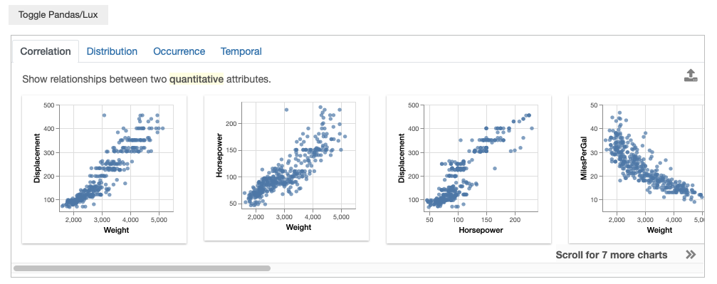
Here, we’ve loaded in the Cars dataset and the visualizations recommended in the widget are in its default settings.
df
By default, visualizations in Lux are rendered using the Altair library. To change the plot configuration in Altair, we need to specify a function that takes an AltairChart as input, performs some chart configurations in Altair, and returns the chart object as an output.
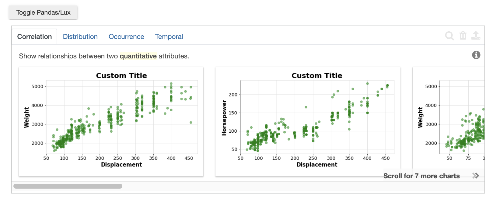
Let’s say that we want to change all the graphical marks of the charts to green and add a custom title. We can define this change_color_add_title function, which configures the chart’s mark as green and adds a custom title to the chart.
lux.config.plotting_backend = "altair"
def change_color_add_title(chart):
    chart = chart.configure_mark(color="green") # change mark color to green
    chart.title = "Custom Title" # add title to chart
    return chart
We then set the global plot configuration of the dataframe by changing the plotting_style property. With the added plotting_style, Lux runs this user-defined function after every Vis is rendered to a chart, allow the user-defined function to override any existing default chart settings.
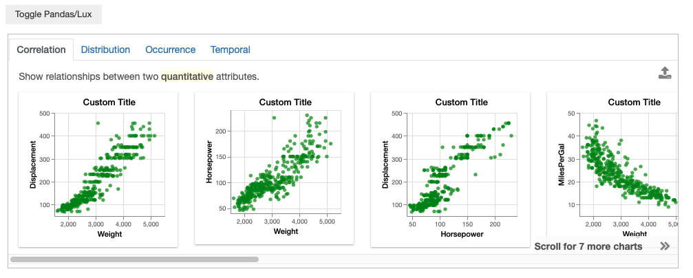
lux.config.plotting_style = change_color_add_title
We now see that the displayed visualizations adopt these new imported settings.
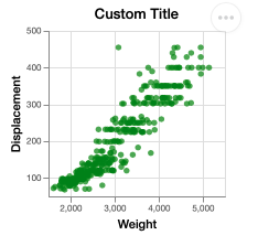
If we click on the visualization for Displacement v.s. Weight and export it. We see that the exported chart now contains code with these additional plot settings at the every end.
# Before running this cell, click on Displacement v.s. Weight vis and export it.
vis = df.exported[0]
print (vis.to_altair())
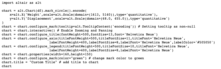
import altair as alt

chart = alt.Chart(df).mark_circle().encode(
    x=alt.X('Weight',scale=alt.Scale(domain=(1613, 5140)),type='quantitative'),
    y=alt.Y('Displacement',scale=alt.Scale(domain=(68.0, 455.0)),type='quantitative')
)
chart = chart.configure_mark(tooltip=alt.TooltipContent('encoding')) # Setting tooltip as non-null
chart = chart.interactive() # Enable Zooming and Panning
chart = chart.configure_title(fontWeight=500,fontSize=13,font='Helvetica Neue')
chart = chart.configure_axis(titleFontWeight=500,titleFontSize=11,titleFont='Helvetica Neue',
                        labelFontWeight=400,labelFontSize=8,labelFont='Helvetica Neue',labelColor='#505050')
chart = chart.configure_legend(titleFontWeight=500,titleFontSize=10,titleFont='Helvetica Neue',
                        labelFontWeight=400,labelFontSize=8,labelFont='Helvetica Neue')
chart = chart.properties(width=160,height=150)
chart = chart.configure_mark(color="green") # change mark color to green
chart.title = "Custom Title" # add title to chart
chart
Similarly, we can change the plot configurations for Matplotlib charts as well. The plotting_style attribute for Matplotlib charts takes in both the fig and ax as parameters. fig handles figure width and other plot size attributes. ax supports changing the chart title and other plot labels and configurations.
lux.config.plotting_backend = "matplotlib"
def change_width_add_title(fig, ax):
    fig.set_figwidth(7)
    ax.set_title("Custom Title")
    return fig, ax
lux.config.plotting_style = change_width_add_title
Moreover, we can set the color and other figure styles using the rcParams attribute of pyplot.
import matplotlib.pyplot as plt
import matplotlib

plt.rcParams['axes.prop_cycle'] = matplotlib.cycler(color='g')
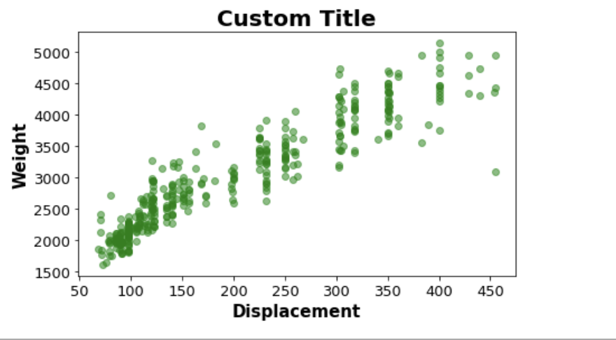
We now see that the displayed visualizations adopt these new imported settings.
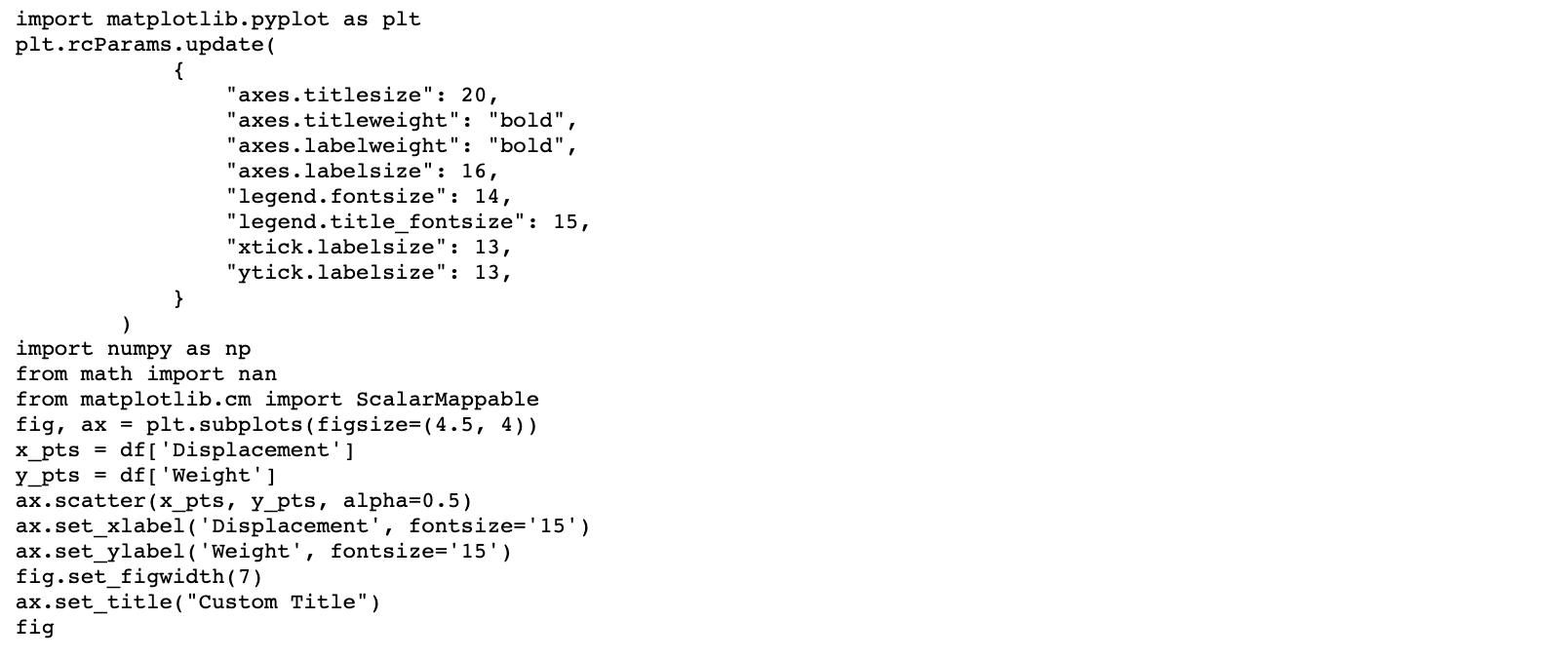
We can also export these Matplotlib charts with the plotting style.
# Before running this cell, click on Displacement v.s. Weight vis and export it.
vis = df.exported[0]
print (vis.to_matplotlib())
import matplotlib.pyplot as plt
plt.rcParams.update(
                        {
                                "axes.titlesize": 20,
                                "axes.titleweight": "bold",
                                "axes.labelweight": "bold",
                                "axes.labelsize": 16,
                                "legend.fontsize": 14,
                                "legend.title_fontsize": 15,
                                "xtick.labelsize": 13,
                                "ytick.labelsize": 13,
                        }
                )
import numpy as np
from math import nan
from matplotlib.cm import ScalarMappable
fig, ax = plt.subplots(figsize=(4.5, 4))
x_pts = df['Displacement']
y_pts = df['Weight']
ax.scatter(x_pts, y_pts, alpha=0.5)
ax.set_xlabel('Displacement', fontsize='15')
ax.set_ylabel('Weight', fontsize='15')
fig.set_figwidth(7)
ax.set_title("Custom Title")
fig
Example #2: Changing Selected Chart Setting
Next, we look at an example of customizing the chart setting for only selected sets of visualizations.
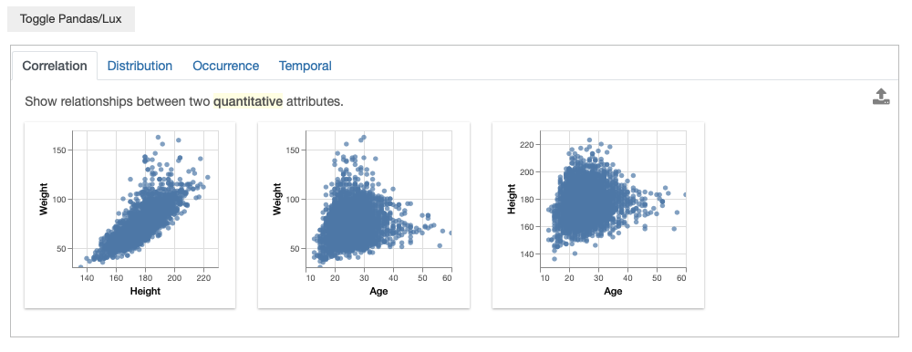
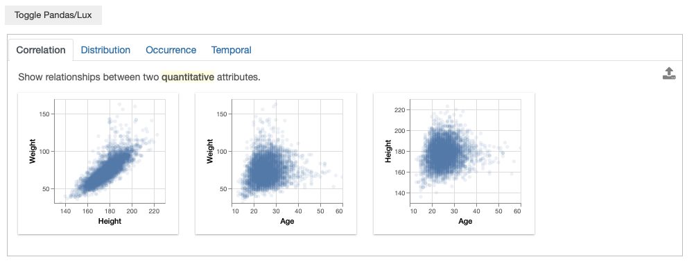
Here, we load in the Olympics dataset and see that the recommended visualization is cluttered with many datapoints.
df = pd.read_csv("../../lux/data/olympic.csv")
df["Year"] = pd.to_datetime(df["Year"], format='%Y') # change pandas dtype for the column "Year" to datetype
df.default_display = "lux"
df
We want to decrease the opacity of scatterplots, but keep the opacity for the other types of visualization as default.
def changeOpacityScatterOnly(chart):
    if chart.mark=='circle':
        chart = chart.configure_mark(opacity=0.1) # lower opacity
    return chart
lux.config.plotting_style = changeOpacityScatterOnly
df
Note
For now, if the visualization has already been rendered before, you will need to run df.expire_recs() to see the updated visualization.
We can modify the scatterplot setting, without changing the settings for the other chart types.